Leray–Hirsch theorem

Reaction–diffusion systems are mathematical models which explain how the concentration of one or more substances distributed in space changes under the influence of two processes: local chemical reactions in which the substances are transformed into each other, and diffusion which causes the substances to spread out over a surface in space.

Reaction–diffusion systems are naturally applied in chemistry. However, the system can also describe dynamical processes of non-chemical nature. Examples are found in biology, geology and physics and ecology. Mathematically, reaction–diffusion systems take the form of semi-linear parabolic partial differential equations. They can be represented in the general form

$\partial _{t}{\boldsymbol {q}}={\underline {\underline {\boldsymbol {D}}}}\,\nabla ^{2}{\boldsymbol {q}}+{\boldsymbol {R}}({\boldsymbol {q}}),$

where each component of the vector q(x,t) represents the concentration of one substance, Template:Uuline is a diagonal matrix of diffusion coefficients, and R accounts for all local reactions. The solutions of reaction–diffusion equations display a wide range of behaviours, including the formation of travelling waves and wave-like phenomena as well as other self-organized patterns like stripes, hexagons or more intricate structure like dissipative solitons.

One-component reaction–diffusion equations

The simplest reaction–diffusion equation concerning the concentration u of a single substance in one spatial dimension,

$\partial _{t}u=D\partial _{x}^{2}u+R(u),$

is also referred to as the KPP (Kolmogorov-Petrovsky-Piskounov) equation. If the reaction term vanishes, then the equation represents a pure diffusion process. The corresponding equation is Fick's second law. The choice R(u) = u(1-u) yields Fisher's equation that was originally used to describe the spreading of biological populations, the Newell-Whitehead-Segel equation with R(u) = u(1 − u²) to describe Rayleigh-Benard convection, the more general Zeldovich equation with R(u) = u(1 − u)(u − α) and 0 < α < 1 that arises in combustion theory, and its particular degenerate case with R(u) = u² − u³ that is sometimes referred to as the Zeldovich equation as well.

The dynamics of one-component systems is subject to certain restrictions as the evolution equation can also be written in the variational form

$\partial _{t}u=-{\frac {\delta {\mathfrak {L}}}{\delta u}}$

and therefore describes a permanent decrease of the "free energy" ${\mathfrak {L}}$ given by the functional

${\mathfrak {L}}=\int \limits _{-\infty }^{\infty }\left[{\frac {D}{2}}(\partial _{x}u)^{2}-V(u)\right]{\text{d}}x$

with a potential V(u) such that R(u)=dV(u)/du.

A travelling wave front solution for Fisher's equation.

In systems with more than one stationary homogeneous solution, a typical solution is given by travelling fronts connecting the homogeneous states. These solutions move with constant speed without changing their shape and are of the form u(x, t) = û(ξ) with ξ = x − ct, where c is the speed of the travelling wave. Note that while travelling waves are generically stable structures, all non-monotonous stationary solutions (e.g. localized domains composed of a front-antifront pair) are unstable. For c = 0, there is a simple proof for this statement: if u₀(x) is a stationary solution and u=u₀(x) + ũ(x, t) is an infinitesimally perturbed solution, linear stability analysis yields the equation

$\partial _{t}{\tilde {u}}=D\partial _{x}^{2}{\tilde {u}}-U(x){\tilde {u}},\quad U(x)=-R^{\prime }(u)|_{u=u_{0}(x)}.$

With the ansatz ũ = ψ(x)exp(−λt) we arrive at the eigenvalue problem

${\hat {H}}\psi =\lambda \psi ,\qquad {\hat {H}}=-D\partial _{x}^{2}+U(x),$

of Schrödinger type where negative eigenvalues result in the instability of the solution. Due to translational invariance ψ = ∂_xu₀(x) is a neutral eigenfunction with the eigenvalue λ = 0, and all other eigenfunctions can be sorted according to an increasing number of knots with the magnitude of the corresponding real eigenvalue increases monotonically with the number of zeros. The eigenfunction ψ = ∂_x u₀(x) should have at least one zero, and for a non-monotonic stationary solution the corresponding eigenvalue λ = 0 cannot be the lowest one, thereby implying instability.

To determine the velocity c of a moving front, one may go to a moving coordinate system and look at stationary solutions:

$D\partial _{\xi }^{2}{\hat {u}}(\xi )+c\partial _{\xi }{\hat {u}}(\xi )+R({\hat {u}}(\xi ))=0.$

This equation has a nice mechanical analogue as the motion of a mass D with position û in the course of the "time" ξ under the force R with the damping coefficient c which allows for a rather illustrative access to the construction of different types of solutions and the determination of c.

When going from one to more space dimensions, a number of statements from one-dimensional systems can still be applied. Planar or curved wave fronts are typical structures, and a new effect arises as the local velocity of a curved front becomes dependent on the local radius of curvature (this can be seen by going to polar coordinates). This phenomenon leads to the so-called curvature-driven instability.

Two-component reaction–diffusion equations

Two-component systems allow for a much larger range of possible phenomena than their one-component counterparts. An important idea that was first proposed by Alan Turing is that a state that is stable in the local system should become unstable in the presence of diffusion.

A linear stability analysis however shows that when linearizing the general two-component system

$\left({\begin{array}{c}\partial _{t}u\\\partial _{t}v\end{array}}\right)=\left({\begin{array}{cc}D_{u}&0\\0&D_{v}\end{array}}\right)\left({\begin{array}{c}\partial _{xx}u\\\partial _{xx}v\end{array}}\right)+\left({\begin{array}{c}F(u,v)\\G(u,v)\end{array}}\right)$

a plane wave perturbation

${\tilde {\boldsymbol {q}}}_{\boldsymbol {k}}({\boldsymbol {x}},t)=\left({\begin{array}{c}{\tilde {u}}(t)\\{\tilde {v}}(t)\end{array}}\right)e^{i{\boldsymbol {k}}\cdot {\boldsymbol {x}}}$

of the stationary homogeneous solution will satisfy

$\left({\begin{array}{c}\partial _{t}{\tilde {u}}_{\boldsymbol {k}}(t)\\\partial _{t}{\tilde {v}}_{\boldsymbol {k}}(t)\end{array}}\right)=-k^{2}\left({\begin{array}{c}D_{u}{\tilde {u}}_{\boldsymbol {k}}(t)\\D_{v}{\tilde {v}}_{\boldsymbol {k}}(t)\end{array}}\right)+{\boldsymbol {R}}^{\prime }\left({\begin{array}{c}{\tilde {u}}_{\boldsymbol {k}}(t)\\{\tilde {v}}_{\boldsymbol {k}}(t)\end{array}}\right).$

Turing's idea can only be realized in four equivalence classes of systems characterized by the signs of the Jacobian R' of the reaction function. In particular, if a finite wave vector k is supposed to be the most unstable one, the Jacobian must have the signs

$\left({\begin{array}{cc}+&-\\+&-\end{array}}\right),\quad \left({\begin{array}{cc}+&+\\-&-\end{array}}\right),\quad \left({\begin{array}{cc}-&+\\-&+\end{array}}\right),\quad \left({\begin{array}{cc}-&-\\+&+\end{array}}\right).$

This class of systems is named activator-inhibitor system after its first representative: close to the ground state, one component stimulates the production of both components while the other one inhibits their growth. Its most prominent representative is the FitzHugh–Nagumo equation

${\begin{aligned}\partial _{t}u&=d_{u}^{2}\,\nabla ^{2}u+f(u)-\sigma v,\\\tau \partial _{t}v&=d_{v}^{2}\,\nabla ^{2}v+u-v\end{aligned}}$

with ƒ(u) = λu − u³ − κ which describes how an action potential travels through a nerve. Here, d_u, d_v, τ, σ and λ are positive constants.

When an activator-inhibitor system undergoes a change of parameters, one may pass from conditions under which a homogeneous ground state is stable to conditions under which it is linearly unstable. The corresponding bifurcation may be either a Hopf bifurcation to a globally oscillating homogeneous state with a dominant wave number k = 0 or a Turing bifurcation to a globally patterned state with a dominant finite wave number. The latter in two spatial dimensions typically leads to stripe or hexagonal patterns.

• Subcritical Turing bifurcation: formation of a hexagonal pattern from noisy initial conditions in the above two-component reaction-diffusion system of Fitzhugh-Nagumo type.
• 

  Noisy initial conditions at t = 0.

• 

  State of the system at t = 10.

• 

  Almost converged state at t = 100.

For the Fitzhugh-Nagumo example, the neutral stability curves marking the boundary of the linearly stable region for the Turing and Hopf bifurcation are given by

${\begin{aligned}q_{\text{n}}^{H}(k):&{}\quad {\frac {1}{\tau }}+(d_{u}^{2}+{\frac {1}{\tau }}d_{v}^{2})k^{2}&=f^{\prime }(u_{h}),\\[6pt]q_{\text{n}}^{T}(k):&{}\quad {\frac {\kappa }{1+d_{v}^{2}k^{2}}}+d_{u}^{2}k^{2}&=f^{\prime }(u_{h}).\end{aligned}}$

If the bifurcation is subcritical, often localized structures (dissipative solitons) can be observed in the hysteretic region where the pattern coexists with the ground state. Other frequently encountered structures comprise pulse trains (also known as periodic travelling waves), spiral waves and target patterns. These three solution types are also generic features of two- (or more-) component reaction-diffusion equations in which the local dynamics have a stable limit cycle

• Other patterns found in the above two-component reaction-diffusion system of Fitzhugh-Nagumo type.
• 

  Rotating spiral.

• 

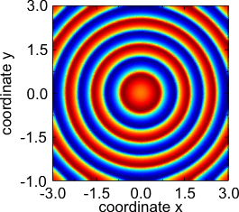
  Target pattern.

• 

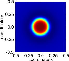
  Stationary localized pulse (dissipative soliton).

Three- and more-component reaction–diffusion equations

For a variety of systems, reaction-diffusion equations with more than two components have been proposed, e.g. as models for the Belousov-Zhabotinsky reaction, , for blood clotting or planar gas discharge systems.

It is known that systems with more components allow for a variety of phenomena not possible in systems with one or two components (e.g. stable running pulses in more than one spatial dimension without global feedback),. An introduction and systematic overview of the possible phenomena in dependence on the properties of the underlying system is given in.

Applications and universality

In recent times, reaction–diffusion systems have attracted much interest as a prototype model for pattern formation. The above-mentioned patterns (fronts, spirals, targets, hexagons, stripes and dissipative solitons) can be found in various types of reaction-diffusion systems in spite of large discrepancies e.g. in the local reaction terms. It has also been argued that reaction-diffusion processes are an essential basis for processes connected to morphogenesis in biology and may even be related to animal coats and skin pigmentation. DTZ's public sale group in Singapore auctions all forms of residential, workplace and retail properties, outlets, homes, lodges, boarding homes, industrial buildings and development websites. Auctions are at present held as soon as a month.

We will not only get you a property at a rock-backside price but also in an space that you've got longed for. You simply must chill out back after giving us the accountability. We will assure you 100% satisfaction. Since we now have been working in the Singapore actual property market for a very long time, we know the place you may get the best property at the right price. You will also be extremely benefited by choosing us, as we may even let you know about the precise time to invest in the Singapore actual property market.

The Hexacube is offering new ec launch singapore business property for sale Singapore investors want to contemplate. Residents of the realm will likely appreciate that they'll customize the business area that they wish to purchase as properly. This venture represents one of the crucial expansive buildings offered in Singapore up to now. Many investors will possible want to try how they will customise the property that they do determine to buy by means of here. This location has offered folks the prospect that they should understand extra about how this course of can work as well.

Singapore has been beckoning to traders ever since the value of properties in Singapore started sky rocketing just a few years again. Many businesses have their places of work in Singapore and prefer to own their own workplace area within the country once they decide to have a everlasting office. Rentals in Singapore in the corporate sector can make sense for some time until a business has discovered a agency footing. Finding Commercial Property Singapore takes a variety of time and effort but might be very rewarding in the long term.

is changing into a rising pattern among Singaporeans as the standard of living is increasing over time and more Singaporeans have abundance of capital to invest on properties. Investing in the personal properties in Singapore I would like to applaud you for arising with such a book which covers the secrets and techniques and tips of among the profitable Singapore property buyers. I believe many novice investors will profit quite a bit from studying and making use of some of the tips shared by the gurus." – Woo Chee Hoe Special bonus for consumers of Secrets of Singapore Property Gurus Actually, I can't consider one other resource on the market that teaches you all the points above about Singapore property at such a low value. Can you? Condominium For Sale (D09) – Yong An Park For Lease

In 12 months 2013, c ommercial retails, shoebox residences and mass market properties continued to be the celebrities of the property market. Models are snapped up in report time and at document breaking prices. Builders are having fun with overwhelming demand and patrons need more. We feel that these segments of the property market are booming is a repercussion of the property cooling measures no.6 and no. 7. With additional buyer's stamp responsibility imposed on residential properties, buyers change their focus to commercial and industrial properties. I imagine every property purchasers need their property funding to understand in value. Other applications of reaction-diffusion equations include ecological invasions, spread of epidemics, tumour growth and wound healing. Another reason for the interest in reaction-diffusion systems is that although they are nonlinear partial differential equations, there are often possibilities for an analytical treatment.

Experiments

Well-controllable experiments in chemical reaction-diffusion systems have up to now been realized in three ways. First, gel reactors or filled capillary tubes may be used. Second, temperature pulses on catalytic surfaces have been investigated. Third, the propagation of running nerve pulses is modelled using reaction-diffusion systems.

Aside from these generic examples, it has turned out that under appropriate circumstances electric transport systems like plasmas or semiconductors can be described in a reaction-diffusion approach. For these systems various experiments on pattern formation have been carried out.

See also

Organisational Psychologist Alfonzo Lester from Timmins, enjoys pinochle, property developers in new launch singapore property and textiles. Gets motivation through travel and just spent 7 days at Alejandro de Humboldt National Park.

• Autowave
• Diffusion-controlled reaction
• Chemical kinetics
• Phase space method
• Autocatalytic reactions and order creation
• Pattern formation
• Patterns in nature
• Periodic travelling wave
• Stochastic geometry
• MClone

42 year-old Environmental Consultant Merle Eure from Hudson, really loves snowboarding, property developers in new launch ec singapore and cosplay. Maintains a trip blog and has lots to write about after visiting Chhatrapati Shivaji Terminus (formerly Victoria Terminus).

References

43 year old Petroleum Engineer Harry from Deep River, usually spends time with hobbies and interests like renting movies, property developers in singapore new condominium and vehicle racing. Constantly enjoys going to destinations like Camino Real de Tierra Adentro.

External links

• Java applet showing a reaction–diffusion simulation
• Another applet showing Gray-Scott reaction-diffusion.
• Java applet Uses reaction-diffusion to simulate pattern formation in several snake species.
• Gallery of reaction-diffusion images and movies.
• TexRD software random texture generator based on reaction-diffusion for graphists and scientific use
• Reaction-Diffusion by the Gray-Scott Model: Pearson's parameterization a visual map of the parameter space of Gray-Scott reaction diffusion.
• A Thesis on reaction-diffusion patterns with an overview of the field
• ReDiLab - Reaction Diffusion Laboratory Flash & GPU based application simulating Belousov-Zhabotinsky, Gray Scott, Willamowski–Rössler and FitzHugh-Nagumo with full source code.