File:Aliasing between a positive and a negative frequency.png
Jump to navigation
Jump to search
No higher resolution available.
Aliasing_between_a_positive_and_a_negative_frequency.png (694 × 452 pixels, file size: 44 KB, MIME type: image/png)
Summary
| Description |
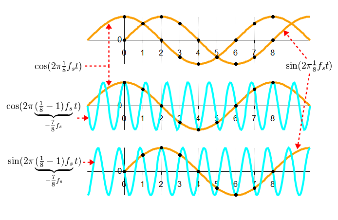
English: This figure depicts two complex sinusoids, colored gold and cyan, that fit the same sets of real and imaginary sample points. They are thus aliases of each other when sampled at the rate (fs) indicated by the grid lines. The gold-colored function depicts a positive frequency, because its real part (the cos function) leads its imaginary part by 1/4 of one cycle. The cyan function depicts a negative frequency, because its real part lags the imaginary part. |
|||
| Date | ||||
| Source | Own work | |||
| Author | Bob K | |||
| Permission (Reusing this file) |
I, the copyright holder of this work, hereby publish it under the following license:
|
|||
| Other versions |
Derivative works of this file: Aliasing between a positive and a negative frequency.svg
|
|||
| PNG development | This PNG graphic was created with LibreOffice. |
|||
| Octave/gnuplot source | click to expand
This graphic was created with the help of the following Octave script: graphics_toolkit gnuplot
gold = [251 159 3]/256; % arbitrary color choice
sam_per_sec = 1;
T = 1/sam_per_sec; % sample interval
dt = T/20; % time-resolution of continuous functions
cycle_per_sec = sam_per_sec/8; % sam_per_sec = 8 * cycle_per_sec (satisfies Nyquist)
figure
subplot(3,1,1)
xlim([-2 10])
ylim([-1.3 1.3])
% Plot cosine function
start_time_sec = -2;
stop_time_sec = 10;
x = start_time_sec : dt : stop_time_sec;
y = cos(2*pi*cycle_per_sec*x);
plot(x, y, "color", gold, "linewidth", 4)
box off % no border around plot please
hold on % same axes for next 3 plots
% Plot sine function
start_time_sec = 0;
stop_time_sec = 10;
x = start_time_sec : dt : stop_time_sec;
y = sin(2*pi*cycle_per_sec*x);
plot(x, y, "color", gold, "linewidth", 4)
% Sample cosine function at sample-rate (1/T)
start_time_sec = 0;
stop_time_sec = 8;
x = start_time_sec : T : stop_time_sec;
y = cos(2*pi*cycle_per_sec*x);
plot(x, y, "color", "black", ".")
% Sample sine function
y = sin(2*pi*cycle_per_sec*x);
plot(x, y, "color", "black", ".")
set(gca, "xaxislocation", "origin")
set(gca, "yaxislocation", "origin")
set(gca, "xgrid", "on");
set(gca, "ygrid", "off");
set(gca, "ytick", [0]);
set(gca, "xtick", [0:8]);
subplot(3,1,2)
xlim([-2 10])
ylim([-1.3 1.3])
cycle_per_sec2 = cycle_per_sec - sam_per_sec; % negative frequency
% Re-plot same cosine function on new axes
start_time_sec = -2;
stop_time_sec = 10;
x = start_time_sec : dt : stop_time_sec;
y = cos(2*pi*cycle_per_sec*x);
plot(x, y, "color", gold, "linewidth", 4)
box off
hold on
% Plot other cosine function
start_time_sec = -2;
stop_time_sec = 10;
x = start_time_sec : dt : stop_time_sec;
y = cos(2*pi*cycle_per_sec2*x);
plot(x, y, "color", "cyan", "linewidth", 4)
% Sample cosine functions at sample-rate (1/T)
start_time_sec = 0;
stop_time_sec = 8;
x = start_time_sec : T : stop_time_sec;
y = cos(2*pi*cycle_per_sec*x);
plot(x, y, "color", "black", ".")
set(gca, "xaxislocation", "origin")
set(gca, "yaxislocation", "origin")
set(gca, "xgrid", "on");
set(gca, "ygrid", "off");
set(gca, "ytick", [0]);
set(gca, "xtick", [0:8]);
subplot(3,1,3)
xlim([-2 10])
ylim([-1.3 1.3])
% Re-plot original sine function on new axes
start_time_sec = 0;
stop_time_sec = 10;
x = start_time_sec : dt : stop_time_sec;
y = sin(2*pi*cycle_per_sec*x);
plot(x, y, "color", gold, "linewidth", 4)
box off
hold on
% Plot other sine function
start_time_sec = -2;
stop_time_sec = 10;
x = start_time_sec : dt : stop_time_sec;
y = sin(2*pi*cycle_per_sec2*x);
plot(x, y, "color", "cyan", "linewidth", 4)
% Sample sine functions at sample-rate (1/T)
start_time_sec = 0;
stop_time_sec = 8;
x = start_time_sec : T : stop_time_sec;
y = sin(2*pi*cycle_per_sec*x);
plot(x, y, "color", "black", ".")
set(gca, "xaxislocation", "origin")
set(gca, "yaxislocation", "origin")
set(gca, "xgrid", "on");
set(gca, "ygrid", "off");
set(gca, "ytick", [0]);
set(gca, "xtick", [0:8]);
|


File history
Click on a date/time to view the file as it appeared at that time.
| Date/Time | Thumbnail | Dimensions | User | Comment | |
|---|---|---|---|---|---|
| current | 07:26, 27 March 2013 | | 694 × 452 (44 KB) | wikimediacommons>Bob K | User created page with UploadWizard |
File usage
There are no pages that use this file.