File:Gauss Newton illustration.png
Jump to navigation
Jump to search

Size of this preview: 743 × 599 pixels. Other resolutions: 298 × 240 pixels | 595 × 480 pixels | 952 × 768 pixels | 1,269 × 1,024 pixels | 1,532 × 1,236 pixels.
Original file (1,532 × 1,236 pixels, file size: 53 KB, MIME type: image/png)
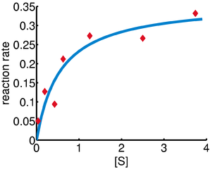
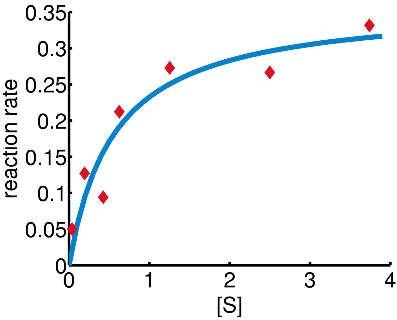
| Description | Illustration of Gauss-Newton applied to a curve-fitting problem with noisy data. What is plotted is the best fit curve versus the data with the fitting parameters obtained via Gauss-Newton. |
| Date | (UTC) |
| Source | self-made with Matlab |
| Author | Oleg Alexandrov |
Source code
function [X, Y] = main()

   f=inline('beta1*x/(beta2+x)', 'beta1', 'beta2', 'x');
   f1=inline('x/(beta2+x)', 'beta1', 'beta2', 'x');
   f2=inline('-beta1*x/(beta2+x)^2', 'beta1', 'beta2', 'x');

   X = [0.038 	0.194 	    0.425 	0.626 	1.253 	2.500 	3.740];
   Y = [0.05    0.127       0.094    0.2122    0.2729    0.2665    0.3317];

   beta10 = 0.9; beta20 = 0.2;

   m = length(X);
   R = zeros(m, 1);
   J = zeros(m, 2);

   v = [beta10, beta20]';

   for k=0:10 % iterate

      for i=1:length(X)
	 R(i)    = Y(i) - f (beta10, beta20, X(i));
	 J(i, 1) =       -f1(beta10, beta20, X(i));
	 J(i, 2) =       -f2(beta10, beta20, X(i));
      end

      disp(sprintf('%d %0.9g %0.9g %0.9g', k, v(1), v(2), norm(R)));

      v = v - (J'*J)\(J'*R);


      beta10 = v(1);
      beta20 = v(2);

   end

   % KSmrq's colors
   red=[0.867 0.06 0.14];
   blue = [0, 129, 205]/256;
   green = [0, 200,  70]/256;
   black = [0, 0, 0];
   white = 0.99*[1, 1, 1];
   gray = 0.8*white;

   fs = 30;
   lw = 7;

   figure(1); clf; hold on;
   set(gca, 'fontsize', fs);

   Hx=xlabel('[S]')
   set(gca, 'linewidth', lw/2);

   Hy=ylabel('reaction rate');


   hold on; %axis equal;

   h=0.1;
   xs = 0; xl = max(X)+0.2;
   Xe = xs:h:xl;
   Ye = 0*Xe;
   for i=1:length(Xe)
      Ye(i) = f(beta10, beta20, Xe(i));
   end
   plot(Xe, Ye, 'color', blue, 'linewidth', lw);

   for i=1:length(X)
      plot(X(i), Y(i), 'color', red, 'marker', 'd', 'linewidth', lw);
   end


   axis([0 4 0 0.35]);
   set(gca, 'XTick', [0 1 2 3 4]);
   set(gca, 'YTick', [0 0.05 0.1 0.15 0.2 0.25 0.3 0.35]);

   saveas(gcf, 'Gauss_Newton_illustration.eps', 'psc2'); % save as eps
   return
| I, the copyright holder of this work, release this work into the public domain. This applies worldwide. In some countries this may not be legally possible; if so: I grant anyone the right to use this work for any purpose, without any conditions, unless such conditions are required by law. |

|
This math image could be re-created using vector graphics as an SVG file. This has several advantages; see Commons:Media for cleanup for more information. If an SVG form of this image is available, please upload it and afterwards replace this template with
{{vector version available|new image name}}.
It is recommended to name the SVG file “Gauss Newton illustration.svg”—then the template Vector version available (or Vva) does not need the new image name parameter. |
File history
Click on a date/time to view the file as it appeared at that time.
| Date/Time | Thumbnail | Dimensions | User | Comment | |
|---|---|---|---|---|---|
| current | 23:36, 20 April 2008 | | 1,532 × 1,236 (53 KB) | wikimediacommons>Oleg Alexandrov | {{Information |Description=Illustration of en:Gauss-Newton algorithm |Source=self-made with Matlab |Date=~~~~~ |Author= Oleg Alexandrov |Permission= see below |other_versions= }} ==Source code== <source lang="matlab"> funct |
File usage
The following page uses this file: