File:Master equation unravelings.svg
Jump to navigation
Jump to search

Size of this PNG preview of this SVG file: 720 × 540 pixels. Other resolutions: 320 × 240 pixels | 640 × 480 pixels | 1,024 × 768 pixels | 1,280 × 960 pixels | 2,560 × 1,920 pixels.
Original file (SVG file, nominally 720 × 540 pixels, file size: 453 KB)
Summary
| Description |
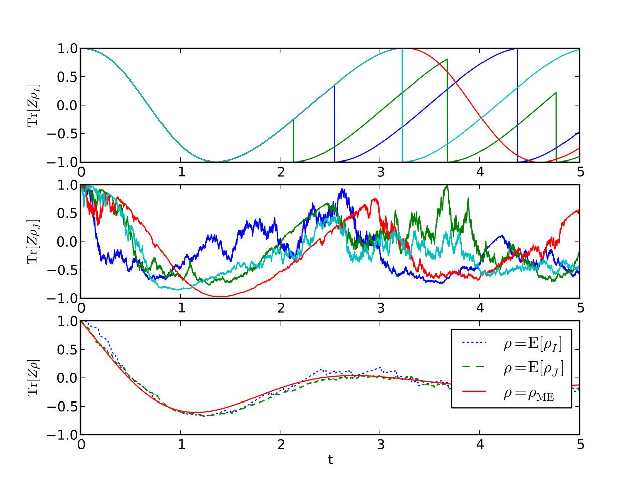
English: Plot of the evolution of the z-component of the Bloch vector of a two-level atom coupled to the electromagnetic field undergoing damped Rabi oscillations. The top plot shows the quantum trajectory for the atom for photon-counting measurements performed on the electromagnetic field, the middle plot shows the same for homodyne detection, and the bottom plot compares the previous two measurement choices (each averaged over 32 trajectories) with the unconditioned evolution given by the master equation. |
| Date | |
| Source | Own work |
| Author | Azaghal of Belegost |
W3C-validity not checked.
Source code
| Source Code in python: |
|---|
import numpy as np
import matplotlib.pyplot as plt
import sys
import random
from math import pi, cos, sin, sqrt

# Pauli matrices
X = np.matrix([[0. + 0.j, 1. + 0.j], [1. + 0.j, 0. + 0.j]])
Y = np.matrix([[0. + 0.j, 0. - 1.j], [0. + 1.j, 0. + 0.j]])
Z = np.matrix([[1. + 0.j, 0. + 0.j], [0. + 0.j, -1 + 0.j]])
Id = np.matrix([[1. + 0.j, 0. + 0.j], [0. + 0.j, 1. + 0.j]])

# Program parameters
timesteps = 1e4
final_time = 5
timestep = final_time/timesteps

# Evolution parameters
H = 1*X
g = 1
L = sqrt(g)*(X - 1.j*Y)/2

# Initial Bloch vector parameters
r = 1
theta = 0
phi = 0
initial_state = 0.5*(Id + r*(cos(theta)*Z + sin(theta)*(cos(phi)*X +
                     sin(phi)*Y)))
trials = 32

def Commutator(A, B):
    return A*B - B*A

def Diffusion(op, state):
    return op*state*op.H - 0.5*(op.H*op*state + state*op.H*op)

def Time_Deriv(hamiltonian, lindblad, state):
    return -1.j*Commutator(hamiltonian, state) + Diffusion(lindblad, state)

def Vacuum_SME_Evol(hamiltonian, lindblad, state, timestep):
    state_trace = np.trace(state*lindblad.H*lindblad)
    E_N = state_trace*timestep
    d_state = 0.5*timestep*(2*state*state_trace - lindblad.H*lindblad*state -
                            state*lindblad.H*lindblad)
    if random.uniform(0, 1) < E_N:
        d_state += lindblad*state*lindblad.H/state_trace - state
    else:
        d_state += -1.j*Commutator(hamiltonian, state)*timestep
    return d_state

def H_supop(op, state):
    return op*state + state*op.H - np.trace((op + op.H)*state)*state

def Homodyne_Vac_SME_Evol(hamiltonian, lindblad, state, timestep):
    d_state = (Diffusion(lindblad, state) -
               1.j*Commutator(hamiltonian, state))*timestep
    state_trace = np.trace(lindblad*state + state*lindblad.H)
    if random.uniform(0, 1) < (1 + sqrt(timestep)*state_trace)/2:
        d_R = sqrt(timestep)
    else:
        d_R = -sqrt(timestep)
    d_state += (d_R - state_trace*timestep)*H_supop(lindblad, state)
    return d_state

def main():
    state = initial_state
    E_z = []
    states = []
    times = np.arange(0, final_time, timestep)
# Calculate the trajectory from the master equation
    for time in times:
        states.append(state)
        E_z.append(np.trace(Z*state))
        state = state + Time_Deriv(H, L, state)*timestep

    cond_E_z = []
    hom_E_z = []
    test_var = pi
    cond_states = []
    hom_states = []
    avg_E_z = []
    avg_hom_E_z = []
# Calculate the conditional evolution for a number of trials
    for trial in range(trials):
        cond_state = initial_state
        cond_states.append([])
        cond_E_z.append([])
        hom_state = initial_state
        hom_states.append([])
        hom_E_z.append([])
        for time in times:
            cond_states[trial].append(cond_state)
            cond_E_z[trial].append(np.trace(Z*cond_state))
            cond_state = cond_state + Vacuum_SME_Evol(H, L, cond_state,
                                                      timestep)
            hom_states[trial].append(hom_state)
            hom_E_z[trial].append(np.trace(Z*hom_state))
            hom_state = hom_state + Homodyne_Vac_SME_Evol(H, L, hom_state,
                                                            timestep)

# Calculate the average behavior of the system over all trials
    for i in range(len(times)):
        sum_z = 0
        for cond_E_z_series in cond_E_z:
            sum_z += cond_E_z_series[i]
        avg_E_z.append(sum_z/len(cond_E_z))
        hom_sum_z = 0
        for hom_E_z_series in hom_E_z:
            hom_sum_z += hom_E_z_series[i]
        avg_hom_E_z.append(hom_sum_z/len(hom_E_z))

# Plot photon-counting conditional evolution for Z expectation value
    fig = plt.figure()
    ax1 = fig.add_subplot(311)
    for i in range(min(4, len(cond_E_z))):
        ax1.plot(times, cond_E_z[i])
    plt.axis([0, 5, -1, 1])
    plt.ylabel(r'$\operatorname{Tr}[Z\rho_I]$')

# Plot homodyne conditional evolution for Z expectation value
    ax2 = fig.add_subplot(312)
    for i in range(min(4, len(hom_E_z))):
        ax2.plot(times, hom_E_z[i])
    plt.axis([0, 5, -1, 1])
    plt.ylabel(r'$\operatorname{Tr}[Z\rho_J]$')

# Plot average Z behavior over conditional evolution trials against master
# equation trajectory
    ax3 = fig.add_subplot(313)
    ax3.plot(times, avg_E_z, dash_joinstyle='round', dash_capstyle='round',
        linestyle=':', label=r'$\rho=\operatorname{E}[\rho_I]$')
    ax3.plot(times, avg_hom_E_z, dash_joinstyle='round', dash_capstyle='round',
        linestyle='--', label=r'$\rho=\operatorname{E}[\rho_J]$')
    ax3.plot(times, E_z, linestyle='-', label=r'$\rho=\rho_\mathrm{ME}$')
    ax3.legend()
    plt.axis([0, 5, -1, 1])
    plt.xlabel('t')
    plt.ylabel(r'$\operatorname{Tr}[Z\rho]$')

    plt.savefig('master_eq_unravelings.svg')

if __name__ == '__main__':
    sys.exit(main())
|
Licensing
I, the copyright holder of this work, hereby publish it under the following license:
This file is licensed under the Creative Commons Attribution-Share Alike 3.0 Unported license.
- You are free:
- to share – to copy, distribute and transmit the work
- to remix – to adapt the work
- Under the following conditions:
- attribution – You must give appropriate credit, provide a link to the license, and indicate if changes were made. You may do so in any reasonable manner, but not in any way that suggests the licensor endorses you or your use.
- share alike – If you remix, transform, or build upon the material, you must distribute your contributions under the same or compatible license as the original.
File history
Click on a date/time to view the file as it appeared at that time.
| Date/Time | Thumbnail | Dimensions | User | Comment | |
|---|---|---|---|---|---|
| current | 05:08, 10 December 2013 | | 720 × 540 (453 KB) | wikimediacommons>Azaghal of Belegost | User created page with UploadWizard |
File usage
The following page uses this file: