File:Navier Stokes Laminar.svg
From formulasearchengine
Jump to navigation
Jump to search

Size of this PNG preview of this SVG file: 750 × 600 pixels. Other resolutions: 300 × 240 pixels | 600 × 480 pixels | 960 × 768 pixels | 1,280 × 1,024 pixels | 2,560 × 2,048 pixels | 900 × 720 pixels.
Original file (SVG file, nominally 900 × 720 pixels, file size: 9.37 MB)
This file is from Wikimedia Commons and may be used by other projects. The description on its file description page there is shown below.
Summary
| DescriptionNavier Stokes Laminar.svg |
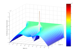
English: SVG illustration of the classic Navier-Stokes obstructed duct problem, which is stated as follows. There is air flowing in the 2-dimensional rectangular duct. In the middle of the duct, there is a point obstructing the flow. We may leverage Navier-Stokes equation to simulate the air velocity at each point within the duct. This plot gives the air velocity component of the direction along the duct. One may refer to [1], in which Eq. (3) is a little simplified version compared with ours. |
| Date | |
| Source |
Own work
The following code leverages some numerical methods to simulate the solution of the 2-dimensional Navier-Stokes equation. We choose the simplified incompressible flow Navier-Stokes Equation as follows: The iterations here are based on the velocity change rate, which is given by Or in X coordinates: |
| Author | IkamusumeFan |
| Other versions |
  |
| SVG development InfoField | This plot was created with Matplotlib. |
| Source code InfoField | Python codefrom __future__ import division
from numpy import arange, meshgrid, sqrt, zeros, sum
import matplotlib.pyplot as plt
from mpl_toolkits.mplot3d import Axes3D
from matplotlib.ticker import ScalarFormatter
from matplotlib import rcParams
rcParams['font.family'] = 'serif'
rcParams['font.size'] = 16
# the layout of the duct laminar
x_max = 5 # duct length
y_max = 1 # duct width
# draw the frames, including the angles and labels
ax = Axes3D(plt.figure(figsize=(10, 8)), azim=20, elev=20)
ax.set_xlabel(r"$x$", fontsize=20)
ax.set_ylabel(r"$y$", fontsize=20)
ax.zaxis.set_rotate_label(False)
ax.set_zlabel(r"$v_x$", fontsize=20, rotation='horizontal')
formatter = ScalarFormatter(useMathText=True)
formatter = ScalarFormatter()
formatter.set_scientific(True)
formatter.set_powerlimits((-2,2))
ax.w_zaxis.set_major_formatter(formatter)
ax.set_xlim([0, x_max])
ax.set_ylim([0, y_max])
# initial speed of the air
ini_v = 3e-3
mu = 1e-5
rho = 1.3
# the acceptable difference when termination
accept_diff = 1e-5
# time interval
time_delta = 1.0
# coordinate interval
delta = 1e-2;
X = arange(0, x_max + delta, delta)
Y = arange(0, y_max + delta, delta)
# number of coordinate points
x_size = len(X) - 1
y_size = len(Y) - 1
Vx = zeros((len(X), len(Y)))
Vy = zeros((len(X), len(Y)))
new_Vx = zeros((len(X), len(Y)))
new_Vy = zeros((len(X), len(Y)))
# initial conditions
Vx[1: x_size - 1, 2:y_size - 1] = ini_v
# start evolution and computation
res = 1 + accept_diff
rounds = 0
alpha = mu/(rho * delta**2)
while (res>accept_diff and rounds<100):
"""
The iterations here are based on the velocity change rate, which
is given by
\frac{\partial v}{\partial t} = \alpha\nabla^2 v - v \cdot \nabla v
with \alpha = \mu/\rho.
"""
new_Vx[2:-2, 2:-2] = Vx[2:-2, 2:-2] + time_delta*(alpha*(Vx[3:-1, 2:-2] +
Vx[2:-2, 3:-1] - 4*Vx[2:-2, 2:-2] + Vx[2:-2, 1:-3] + Vx[1:-3, 2:-2]) -
0.5/delta * (Vx[2:-2, 2:-2] * (Vx[3:-1, 2:-2] - Vx[1:-3, 2:-2]) +
Vy[2:-2, 2:-2]*(Vx[2:-2, 3:-1] - Vx[2:-2, 1:-3])))
new_Vy[2:-2, 2:-2] = Vy[2:-2, 2:-2] + time_delta*(alpha*(Vy[3:-1, 2:-2] +
Vy[2:-2, 3:-1] - 4*Vy[2:-2, 2:-2] + Vy[2:-2, 1:-3] + Vy[1:-3, 2:-2]) -
0.5/delta * (Vy[2:-2, 2:-2] * (Vy[2:-2, 3:-1] - Vy[2:-2, 3:-1]) +
Vx[2:-2, 2:-2]*(Vy[3:-1, 2:-2] - Vy[1:-3, 2:-2])))
rounds = rounds + 1
# copy the new values
Vx[2:-2, 2:-2] = new_Vx[2:-2, 2:-2]
Vy[2:-2, 2:-2] = new_Vy[2:-2, 2:-2]
# set free boundary conditions: dv_x/dx = dv_y/dx = 0.
Vx[-1, 1:-1] = Vx[-3, 1:-1]
Vx[-2, 1:-1] = Vx[-3, 1:-1]
Vy[-1, 1:-1] = Vy[-3, 1:-1]
Vy[-2, 1:-1] = Vy[-3, 1:-1]
# there exists a still object in the plane
Vx[x_size//3:x_size//1.5, y_size//2.0] = 0
Vy[x_size//3:x_size//1.5, y_size//2.0] = 0
# calculate the residual of Vx
res = (Vx[3:-1, 2:-2] + Vx[2:-2, 3:-1] -
Vx[1:-3, 2:-2] - Vx[2:-2, 1:-3])**2
res = sum(res)/(4 * delta**2 * x_size * y_size)
# prepare the plot data
Z = sqrt(Vx**2)
# refine the region boundary
Z[0, 1:-2] = Z[1, 1:-2]
Z[-2, 1:-2] = Z[-3, 1:-2]
Z[-1, 1:-2] = Z[-3, 1:-2]
Y, X = meshgrid(Y, X);
ax.plot_surface(X, Y, Z, rstride=1, cstride=1, cmap="summer", lw=0.1,
edgecolors="k")
plt.savefig("Navier_Stokes_Laminar.svg")
|
Licensing
I, the copyright holder of this work, hereby publish it under the following license:
This file is licensed under the Creative Commons Attribution-Share Alike 4.0 International license.
- You are free:
- to share – to copy, distribute and transmit the work
- to remix – to adapt the work
- Under the following conditions:
- attribution – You must give appropriate credit, provide a link to the license, and indicate if changes were made. You may do so in any reasonable manner, but not in any way that suggests the licensor endorses you or your use.
- share alike – If you remix, transform, or build upon the material, you must distribute your contributions under the same or compatible license as the original.
- ↑ Fan, Chien, and Bei-Tse Chao. "Unsteady, laminar, incompressible flow through rectangular ducts." Zeitschrift für angewandte Mathematik und Physik ZAMP 16, no. 3 (1965): 351-360.
Captions
project
Items portrayed in this file
depicts
File history
Click on a date/time to view the file as it appeared at that time.
| Date/Time | Thumbnail | Dimensions | User | Comment | |
|---|---|---|---|---|---|
| current | 03:06, 15 March 2016 |  | 900 × 720 (9.37 MB) | wikimediacommons>Nicoguaro | Smaller version |
File usage
There are no pages that use this file.


