File:Roundtriptimes.png
Roundtriptimes.png (548 × 573 pixels, file size: 40 KB, MIME type: image/png)
Summary
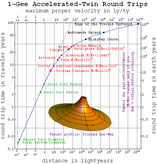
| Description | This plot illustrates how a spaceship capable of 1 g acceleration for 100 years can power a round trip to most anywhere in the visible universe, and back in a lifetime or less. Additional time will have elapsed on earth by the time that you return. This advantage of constant proper acceleration in a relativistic world arises because proper velocity change is proportional to acceleration times the change in map rather than traveler time. As those two begin to differ, the advantage (over the dotted straight line above) emerges. Of course, building a spaceship that can do this is another story. |
| Date | |
| Source | Own work |
| Author | P. Fraundorf |
Added notes

The dotted line shows how far the same round trip would take a traveler if Newtonian physics applied instead. As you can see, the lightspeed limit improves travel prospects for the accelerated traveler even though it makes things worse for the couch-potato who waits at home for the traveler to return. Relativity also can significantly reduce the (still probably exhorbitant) fuel-costs for such trips.
The bronze thrust profile inset above for a 5 traveler-year one-way trip to Proxima Centauri shows how the thrust profile (proportional to cross-sectional area) would vary during the trip. The orange mesh line around the profile corresponds to the thruster turnaround point in the trip. Even longer trips would exponentially decrease traveler time for the trip, but only at the price of a comparably-exponential increase in fuel mass on launch.
The figure at right illustrates how one might apply the equations of constant proper-acceleration to a specific (if fanciful) roundtrip.
Furthermore, it should be noted that, when discussing large distances, the expansion of the universe is important. For example, the edge of the universe (~46 billion light years) can not be reached no matter how fast you accelerate because the cosmic horizon is 16 billion light years.
Deriving unidirectional constant acceleration
For a change of pace from most texts, lets discuss the assumptions needed for a computer to derive the equations of constant acceleration. For equations that work at any speed, we'll also give you some practice treating time as a local instead of as a global variable[1] i.e. as a value connected to readings on a specific clock.
Low-speed (Newtonian) version

If we define coordinate-acceleration a as dv/dt and coordinate-velocity v as dx/dt where x and t are map-position and map-time, respectively, then holding constant the coordinate-acceleration a (which is not the acceleration felt by our traveler at high speeds) allows one to derive the v<<c low-speed constant coordinate-acceleration equations familiar from intro-physics texts for coordinate-velocity v[t] and map-position x[t]. Can you do it?
The following is what Mathematica needs to pull it off:
FullSimplify[
 DSolve[
  {
   v[t] == x'[t],
   a == v'[t],
   x[0] == xo,
   v[0] == vo
  },
 {x[t], v[t]},
 t
 ]
]
Here we've added the intial (t=0) boundary-conditions by defining xo as initial map-position and vo as initial coordinate-velocity to eliminate the two constants of integration. Mathematica's output is:
{{v[t] -> a t + vo, x[t] -> (a t^2)/2 + t vo + xo}}
Thus the equations for constant coordinate-acceleration in one direction might be written:
- ,
- ,


where as usual Δf ≡ ffinal - finitial. Here the first equation tells us how coordinate-velocity v changes with elapsed map-time t, while the second tells us how map-position x changes with map-time t as well as with state-of-motion (the work-energy equation) since work is mαΔx and kinetic energy is K = ½mv2.
In terms of increments instead of differentials for constant unidirectional acceleration, we can therefore also write: a = Δv/Δt = ½Δ(v2)/Δx.
Any-speed version


For equations that work at any speed, we begin by treating the "proper" time τ on the clocks of a traveler as a local-variable, whose value we'd like to figure out relative to the local value of the traveler's position x and time t on the yardsticks and synchronized clocks of a reference map-frame. The space-time Pythagorean theorem or "metric-equation" for flat space-time, namely (cdτ)2 = (cdt)2 - (dx)2 with "lightspeed" constant c, requires that we define "proper" (in addition to "coordinate") values for the velocity and acceleration, as well as for the time, experienced by our traveler.
In particular proper-velocity w (map-distance x per unit proper-time τ) is just w ≡ dx/dτ ≡ c sinh[η], where η is referred to as hyperbolic velocity-angle or rapidity. The frame-invariant proper-acceleration[2] α felt by a traveler equals the "length-contracted" proper-velocity derivative c dη/dτ i.e. constant c times the traveler-time τ derivative of rapidity η. Holding α fixed thus allows one to derive constant proper-acceleration equations that work at any speed for map-position x[τ] and proper-velocity w[τ].
In the above discussion we are using proper-time τ local to the traveler as the independent variable so as to avoid thinking of time as a global variable. Note that unlike coordinate-velocity v≡dx/dt, proper-velocity w≡dx/dτ always equals momentum per unit mass and has no upper limit. Can you figure how map-position x and proper-velocity w = c sinh[η] depend on traveler-time τ, given this information?
The following is what Mathematica needs to pull it off:
FullSimplify[
 DSolve[
  {
   c Sinh[eta[tau]] == x'[tau],
   alpha == c eta'[tau],
   x[0] == xo,
   eta[0] == etao
  },
 {x[tau], eta[tau]}, {tau}
 ]
]
As above we specify two initial (τ=0) conditions, in this case for initial map-position xo and initial rapidity or hyperbolic velocity-angle ηo. The result is:
{
 {
  eta[tau] -> etao + (alpha tau)/c,
  x[tau] -> (alpha xo + c^2 (-Cosh[etao] + Cosh[etao + (alpha tau)/c]))/alpha
 }
}
Note that we also get these bonus relationships: Traveler-speed on the map can be expressed in several ways, including: Lorentz-factor γ ≡ dt/dτ = cosh[η] = Sqrt[1+(w/c)2] = 1/Sqrt[1-(v/c)2], where coordinate-velocity v ≡ w/γ = c tanh[η]. For incremental changes when proper-acceleration is constant and all motion is along that direction we can also write α =Δw/Δt = cΔη/Δτ = c2Δγ/Δx = γ3a.
All of the foregoing assertions are local to the traveler's position in the map-frame of yardsticks and synchronized clocks. If we use those synchronized clocks to define simulaneity between separated events, the above also tells us about traveler motion from the perspective of stationary observers anywhere on the map. Hence these equations are spectacular for exploring constant-acceleration round-trips between stars, as illustrated in the figure at right.
Thus the equations, analogous to the Newtonian ones, for unidirectional constant proper-acceleration at any speed might be written:
- ,
- ,
![{\displaystyle w=c\sinh \left[{\frac {\alpha \tau }{c}}+\eta _{o}\right]=w_{o}+\alpha \int _{0}^{\tau }\gamma [\tau ']d\tau '=w_{o}+\alpha \Delta t\,}](https://wikimedia.org/api/rest_v1/media/math/render/svg/82349738501827ec5919d1c113e8dae9d5b5ced3)
![{\displaystyle x=x_{o}+{\tfrac {c^{2}}{\alpha }}\left(\cosh \left[{\frac {\alpha \tau }{c}}+\eta _{o}\right]-\cosh \left[\eta _{o}\right]\right)=x_{o}+{\frac {c^{2}}{\alpha }}\Delta \gamma }](https://wikimedia.org/api/rest_v1/media/math/render/svg/ecac73b654fdc5ecf73c59d6d803c1a7fa17c109)
where again Δf ≡ ffinal - finitial, and ηo = asinh[wo/c]. Here the first equation tells us how proper-velocity w changes with elapsed traveler-time τ and map-time Δt, while the second tells us how map-position x changes with traveler-time τ as well as with state-of-motion (the work-energy equation) since work is mαΔx and change-in kinetic energy is ΔK = mc2Δγ (given that K = (γ-1)mc2).
At low speeds (w<<c) of course, map & traveler clock times go at the same rate i.e. dt ≈ dτ, the velocity-parameters (coordinate, proper & angle) are essentially the same i.e. v ≈ w ≈ cη, coordinate and proper acceleration are about equal i.e. a ≈ α, and the any-speed equations reduce to the low-speed ones discussed above. P. Fraundorf (talk) 23:53, 1 February 2014 (UTC)
Footnotes
- ↑ P. Fraundorf (2012) "A traveler-centered intro to kinematics", arxiv:1206.2877 [physics.pop-ph].
- ↑ Edwin F. Taylor & John Archibald Wheeler (1966 1st ed. only) Spacetime Physics (W.H. Freeman, San Francisco) ISBN 0-7167-0336-X, Chapter 1 Exercise 51 page 97-98: "Clock paradox III" (pdf archive copy at the Wayback Machine).
Licensing

|
Permission is granted to copy, distribute and/or modify this document under the terms of the GNU Free Documentation License, Version 1.2 or any later version published by the Free Software Foundation; with no Invariant Sections, no Front-Cover Texts, and no Back-Cover Texts. A copy of the license is included in the section entitled GNU Free Documentation License. |
- You are free:
- to share – to copy, distribute and transmit the work
- to remix – to adapt the work
- Under the following conditions:
- attribution – You must give appropriate credit, provide a link to the license, and indicate if changes were made. You may do so in any reasonable manner, but not in any way that suggests the licensor endorses you or your use.
- share alike – If you remix, transform, or build upon the material, you must distribute your contributions under the same or compatible license as the original.
File history
Click on a date/time to view the file as it appeared at that time.
| Date/Time | Thumbnail | Dimensions | User | Comment | |
|---|---|---|---|---|---|
| current | 17:21, 10 January 2010 | | 548 × 573 (40 KB) | wikimediacommons>Unitsphere | Added a short-trip thrust profile to suggest vehicular structures required as well. |
File usage
There are no pages that use this file.